A Star
Lingual Usages
PHYSICS-Astrophysics
Stellar Temperature
Directly measuring a star's temperature using conventional methods is unfeasible due to inherent challenges. Stars exhibit various colors, and these color variations are indicative of distinct continuous spectra. A pivotal insight is derived from the continuous spectra of stars with differing colors, particularly those appearing blue, which prominently exhibit peaks in the shorter wavelength blue range. Notably, a star's coloration is intricately tied to its temperature, as heated objects emit radiation in distinct hues, each corresponding to a specific wavelength and, consequently, temperature. The progression from an initial red glow, signifying relatively lower energy and temperature, to subsequent yellow/green and eventual blue hues signifies increasing temperature.
The quantification of a star's temperature entails an assessment of its continuum, obviating the necessity for a comprehensive spectrum analysis. The more judicious approach involves measuring radiation quantities within specific wavelength intervals, facilitated by filters selectively transmitting defined wavelength ranges. The comparative analysis of radiation intensity across these filters furnishes a quantitative method for ascertaining a star's color, and by extension, its temperature.
Stellar Color
Quantifying a color allows to compare between two almost similar colors, and is applicable in determaining the temperature.
For two standard wavelength ranges, centered at λ1 and λ2. The ratio of the observed brightnesses will be, b(λ1)/b(λ2). This brightness ratio can be converted into a magnitude difference:
\[m_2-m_1=2.5\log(b(\lambda_1)/b(\lambda_2))\]
The quantity m2 – m1 can be defined as the color, measured in magnitudes, corresponding to the wavelength pair, λ1, λ2. For definiteness, if λ2 > λ1. When the temperature increases, b(λ1)/b(λ2) increases. This means that the quantity m2 – m1 increases since the magnitude scale runs backwards. If an object is radiating exactly like a blackbody, then the ratio of brightnesses at any two wavelengths is enough to determine the temperature.
Instead of measuring the intensity of radiation at a wavelength, measuring the amount of energy received in some wavelength interval is possible. Wavelength interval can be controled by using a filter that only passes light in that wavelength range.
Stellar Apparent Brightness:
The apparent brightness depends on two quantities:
- the Intrinsic Luminosity of the star and its distance from us.
- Starlight is also dimmed when it passes through clouds of interstellar dust.) Two identical stars at different distances will have different apparent brightnesses.
Understanding how stars work, requires knowledge of their total luminosities. Therefore requires correcting the apparent brightness for the distance to the star.
Stellar distances
The observed energy flux for a star at a distance d can be calculated by using the its Luminosity L.
If no radiation is absorbed along the way, all the energy per second leaving the surface of the star will cross a sphere at a distance d in the same time. It will just be spread over a larger area. Therefore, the energy per second reaching d is still L, but it is spread over an area of 4πd^2 so the energy flux, f, so the received energy flux falls off Inversely as the square of the distance:
\[f=L/4\pi d^2\]
Distances to astronomical objects are generally hard to determine. Trigonometric parallax can be used in calculating the distances for the nearby stars.
Even the closest stars are too far away to demonstrate parallax when using naked eyes. However, the Earth orbits the Sun at a distance defined to be one astronomical unit (AU). Therefore, a star can be observed in to seperate points, first observation and second observation six months later. The two viewing points are separated by 2 AU.
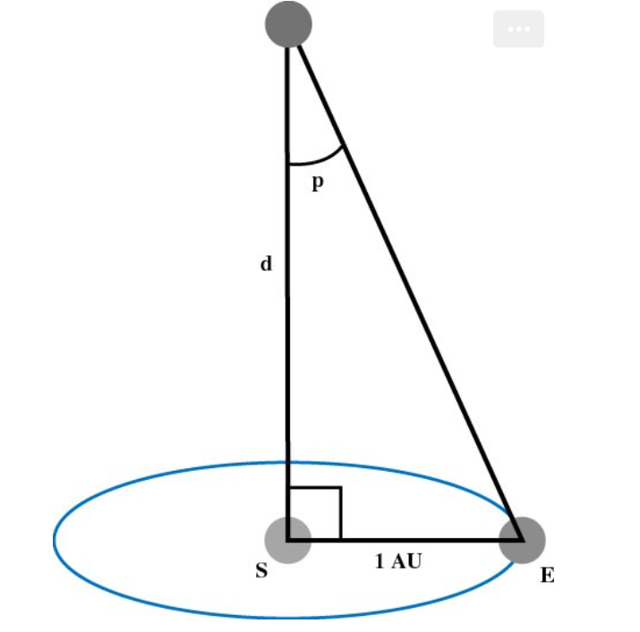
The half of the value of the angle that spans between the two viewing points, is the parallax angle, p.
\[\tan (p)=1 AU/d\]
Given that the distance to the star, d, is much greater than 1 AU in reality, so the parallax angle, p, would normally be very small, and so \(\tan (p)\approx p \)(rad):
\[d=1AU/p\]
Since it is not very convenient measuring such small angles in radians, so it worth to be converted to arc seconds:
\[p\ (“)=2.06\times 10^5 p \ (rad)\]
and: \(1AU=1.50\times 10^8\ km\)
\(d=(1.50\times 10^8)(2.06\times10^5)/p(“)\)\(km/arc \ seconds\)
\(d=(3.09\times 10^{13})/p(“)\)\(km/arc \ seconds\)
This method defines a convenient unit for measuring stellar distances, the parsec (abbreviated pc).
Stellar mass
Measuring the mass of an object (https://app.thebrain.com/brain/cf832a9d-b967-4fdd-92d3-9a9bfc936ab3/0c0e02e9-af96-4efb-9136-fefc21b1f347) involves assessing its gravitational impact on another object. A fortunate opportunity for such measurements arises from binary star (https://app.thebrain.com/brain/cf832a9d-b967-4fdd-92d3-9a9bfc936ab3/4acf883c-4809-4a4e-9599-0bb045682137) systems. Studying the orbits of binary stars provides the opportunity to measure the gravitational forces that the two stars exert on each other, further aiding in determining the masses of the stars.
The mass-temperature relationship on the main sequence imposes a stringent constraint, with cooler stars being less massive and hotter stars being more massive. This relationship determines:
- radius
- temperature
- luminosity: through the mass-luminosity relationship, where the luminosity varies approximately as a power, α, of the mass.
\[L/L _\odot = (M/M_\odot) ^a\]
\(a\) can vary depending on the mass range considered.
Selection Effect
Refers to the bias introduced in a sample of observed objects due to the limitations of the observational method. It arises when certain objects are more likely to be included or excluded from the observed sample based on observational constraints. In the case of studying stars, the selection effect may arise from the fact that brighter stars can be observed at greater distances than fainter ones.
To understand the distribution of stellar masses and proportions of stars of different masses, researchers study the mass function. This involves examining the relative numbers of stars in various mass ranges, providing insights into star formation theories. Due to selection effects that favor brighter stars, obtaining an unbiased sample is challenging. The mass function, which changes over time due to the longer lifespan of low-mass stars, serves as a valuable tool for checking star formation theories. To assess the mix of masses when a cluster forms, scientists examine young clusters, referred to as the initial mass function (IMF). Power laws of the form \(N(m) \sim m^^{-\gamma}\) are often used to fit the data, where \(\gamma\) represents the power-law index.
Stellar sizes
The angular radius of the Sun, Δθ, is 16 arc min. The Sun is at a distance d = 1.50 × 10⁸ km, so its radius, R, is given by:
\[R_\odot =d \tan \Delta \theta\]
The Sun is the only star whose disk subtends an angle larger than the seeing limitations of ground-based telescopes. We therefore need other techniques for determining radii. If we know the luminosity (from its absolute magnitude) and the surface temperature (from the spectral type) of a star, we can calculate its radius using equation
\[L=(\sigma T^4)(4\pi R^2)\]
Solving for the radius gives
\[R=(\frac L{4\pi \sigma T^4})^{1/2}\]
Other Methods:
involve the Moon passing in front of a bright star, and the duration of the star's disappearance provides information about its radius. Diffraction effects during this event contribute to oscillations in light levels, revealing details about the star's radius.
addresses atmospheric seeing fluctuations by collecting short-exposure images of bright stars. By observing interference patterns in light passing through varied atmospheric paths, mathematical reconstruction yields diffraction-limited resolution images.
stars become larger with increasing surface temperature. This is why the luminosity of stars increases with increasing surface temperature at a rate greater than \(T^4\).
Stellar evolution
Stars undergo a repetitive life cycle, beginning with birth, progressing through middle age on the main sequence, and culminating in death, during which they release materials into interstellar space, contributing to the formation of subsequent generations of stars.
The main sequence
Stellar energy sources
When material collapses to form a star, it accumulates gravitational potential energy due to the negative work done by gravity in bringing the material together. The duration of this energy supply is explored by calculating the gravitational potential energy in a uniform sphere.
Gravitational potential energy of a sphere
When dealing with systems comprising a large number of particles, it is convenient to consider a fluid with an average density ρ, rather than individual particles of mass m. The potential energy of a uniform (constant density) sphere is then evaluated, taking into account a sphere with mass M, radius R, and density ρ. Despite real objects deviating from perfect uniformity or sphericity, the results typically differ only by numerical factors of order unity. The calculation involves determining the gravitational potential energy of the specified uniform sphere.
\[M=(4\pi/3)R^3\rho\]
The gravitational potential energy is the work needed to bring all the material from infinity to the final configuration. The final result is independent of the order in which the various parts of the sphere are assembled. To simplify the calculation, the sphere can be conceptualized as being composed of shells. The assembly process involves building the sphere one shell at a time, beginning with the smallest.
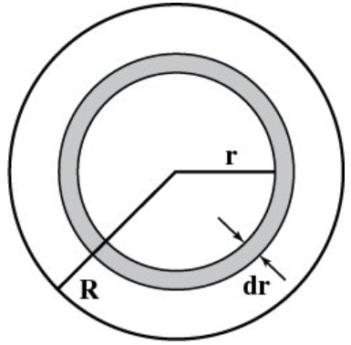
Assuming that shells through radius r have already been assembled, the next step is to calculate the work required to bring in the next shell. The thickness of the shell is represented by dr, and the volume of the thin shell is determined by its surface area multiplied by its thickness.
\[V=\frac 43 \pi r^3\]
so:
\[dV=4\pi r^2dr\]
The mass contained in the shell is:
\[dM=4\pi r^2\rho dr\]
The total mass of material already assembled is:
\[M(r)=(4\pi/3)R^3\rho\]
The importance of the quantity M(r) lies in the fact that the shell ending up at radius r will only experience a net force from material inside it. Even as additional material is brought in from outside this shell, the net force exerted on any particle within the shell by matter outside radius r remains zero. Additionally, for mass within the shell, the mass M(r) exerts a force equivalent to what would be exerted by the same mass concentrated at the center of the sphere.
For any two point masses (the gravitational potential energy relative to infinity) is given by:
\[U=-G\frac{m_1m_2}r \]
If \(m_1 = M(r)\) and \(m_2\) equal the mass of the shell, dM. The work to bring this shell is:
\[dU=-G\frac{M(r)}r dM \]
\[dU=-G\frac{(4\pi/3)r^3\rho}r 4\pi r^2\rho dr \]
\[dU=-G\frac{(4\pi)^2}3 r^4\rho ^2 dr \]
the effect of all the shells equals integration of the quantity dU from r = 0 to r = R:
\[U=\int_0^RdU(r)\]
\[U=-G\frac{(4\pi)^2}3 \rho ^2 \int_0^Rr^4dr\]
\[U=-G\frac{(4\pi)^2}{3\times 5} \rho ^2 R^5\]
But \(M(r)=(4\pi/3)R^3\rho\)so:
\[U=-\frac 35\frac{GM^2}{R} \]
For other shaped objects, the gravitational potential energy is generally proportional to −GM2/R, where R is some average length. The constant of proportionality is generally close to unity.
The thermal energy is (3/2)kT per particle. The total thermal energy is then:
\[K=(3/2)NkT\]
where N is the total number of particles in the cloud. If the mass per particle is m, and the total mass of the cloud is M, then:
\[N=M/m\]
so:
\[K=\frac 32 \frac {kTM}m\]
Gravitational lifetime for a star
It is possible for stars to utilize their stored gravitational potential energy as a source of power. The gravitational lifetime, represented by \(t_g\), is determined by dividing the stored energy by the rate at which it is being lost, which is equivalent to the star's luminosity.
\[t_g=\frac E{dE/dt}\]
The luminosity is defined as:
\[L=\frac {dE}{dt}\]
so:
\[t_g=\frac EL\]
E can be estimated as the negative of the Sun’s current gravitational potential energy:
\[E\approx -U=-(-\frac 35\frac{GM^2}{R}) \]
so:
\[t_g\approx \frac 35\frac{GM^2}{RL} \]
The gravitational lifetime, approximated as \(t_g \approx \frac{3}{5} \frac{GM^2}{RL}\), provides an estimate for the duration of a star's existence powered by gravitational potential energy. This estimation, known as the Kelvin time, is used to calculate the Sun's lifetime, revealing that it is significantly shorter than Earth's geological evidence-based lifetime. This suggests that stars, including the Sun, cannot maintain a stable configuration solely relying on stored gravitational potential energy.
Other energy sources
chemical reactions
An alternative energy source for stars is chemical reactions. Estimating the energy stored in the Sun that could be released through chemical reactions involves considering the binding energy of molecules. Assuming an energy release of about 1 eV per atom, the total chemical energy is calculated as 1 eV multiplied by the total number of atoms in the Sun (M/m). However, the calculated chemical energy is much less than the energy stored in gravitational potential energy, indicating that chemical reactions cannot provide a longer-term energy source for the Sun.
Chemical reactions are dismissed as a viable energy source for the Sun due to the limited energy release per atom, even with highly energetic reactions. The energies associated with chemical reactions are typically a few eV, insufficient to meet the Sun's energy needs.
Nuclear physics
Nuclear building blocks
Nuclear energy for stars
Stellar Old Age
In understanding a star's structure and evolution, its mass is the primary determinant. For main sequence stars, mass dictates both size and temperature. The main sequence lifespan relies on available fuel and its consumption rate, luminosity, both of which are influenced by the star's mass. As a star depletes its fuel, its ultimate fate is also contingent on its mass and initial composition. Vogt's theorem establishes that a star's structure and evolution are entirely determined by its mass and initial composition, a conclusion derived mathematically from the pertinent physical equations.
Evolution off the main sequence
Low mass stars
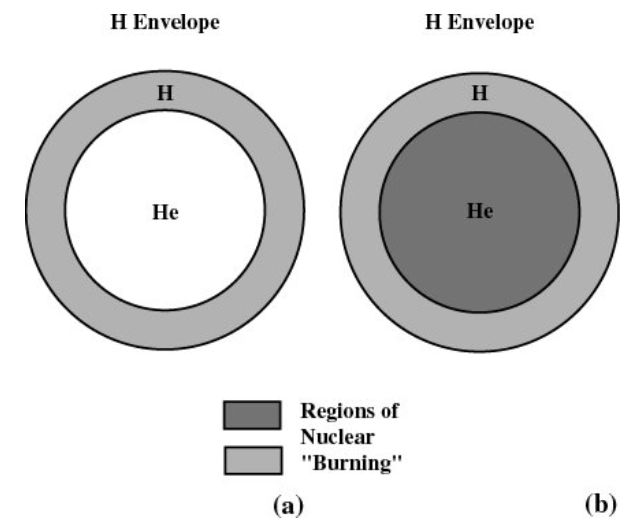
(a) The temperature in the star is not hot enough to fuse the helium in the center, but is hot enough to keep the H in the shell burning. (b) In this star, the temperature is hot enough to keep both burning.
For stars with a mass less than about 5 solar masses, the depletion of hydrogen in the core leads to the formation of helium. However, for lower mass stars, the core temperature is insufficient for helium fusion into heavier elements, despite the presence of ample hydrogen outside the core. Consequently, the core contracts, converting gravitational potential energy into kinetic energy, resulting in core heating. The outer hydrogen layer, just outside the core, becomes hot enough to fuse and forms helium in a hydrogen-burning shell at the core's outer edge. As the core contracts, the energy generation rate in the shell surpasses that of the core during the star's regular lifespan.
Simultaneously, the star's outer layers experience changes as energy transport from the core becomes radiative, leading to outer layer expansion, increased cooling, and a slight rise in luminosity. This shift is depicted on the HR diagram as the star moves rightward and appears as a subgiant. Photon diffusion prevents the surface temperature from dropping too much during this phase.
When the star becomes a red giant, convective energy transport dominates due to a significant negative temperature gradient. The core evolves Concurrently, reaching temperatures of 108 K, enabling the triple-alpha process to fuse helium into carbon. The dense core becomes a degenerate gas, and the sudden release of energy during this process is termed the helium flash. Subsequently, helium fusion stabilizes in a non-degenerate core, accompanied by ongoing hydrogen fusion in the surrounding shell.
After all helium in the core is converted to carbon and oxygen, the core contracts, triggering helium-burning shell development and envelope expansion. The star ascends the giant branch, reaching the asymptotic giant branch on the HR diagram. The star may briefly become a red supergiant and experience oscillations in nuclear energy generation.
High mass stars
More massive stars have a shorter main sequence lifetime compared to lower mass stars. The main sequence lifetime for higher mass stars concludes when the hydrogen in the core is depleted, leading to core contraction and the onset of helium fusion into heavier elements. Unlike lower mass stars, helium fusion in more massive stars occurs steadily without the core becoming degenerate. Subsequently, the star features a helium-burning core surrounded by a hydrogen-burning shell.
After helium exhaustion, the temperature rises sufficiently for carbon and oxygen fusion, resulting in a core with carbon- and oxygen-burning, surrounded by a helium-burning shell and a hydrogen-burning shell. As heavier elements accumulate, the core develops more layers.
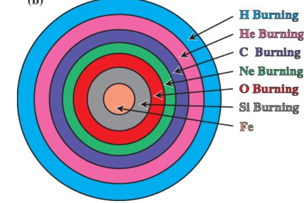
In the core, there is a succession of shells of different composition. Each shell has exhausted the fuels that are still burning in shells farther out.
The increasing luminosity of the core causes the outer layers of the star to expand. Despite cooling, the size grows enough for overall luminosity to increase. The envelope becomes convective, constrained by the adiabatic lapse rate to accommodate the temperature difference between the core and surface. When the radius reaches about 103 times the solar radius, the star is referred to as a red supergiant.
Cepheid variables
Variable stars
Variable stars exhibit brightness fluctuations over time. Eclipsing binaries, where stars eclipse each other, and intrinsic changes within stars contribute to this variability. Naming conventions for bright stars involve Greek letters followed by the constellation name's Latin genitive form. Variable stars are designated by letters (R, S, etc.) in order of discovery within a constellation, and numbers or letters with a "V" for additional designations.
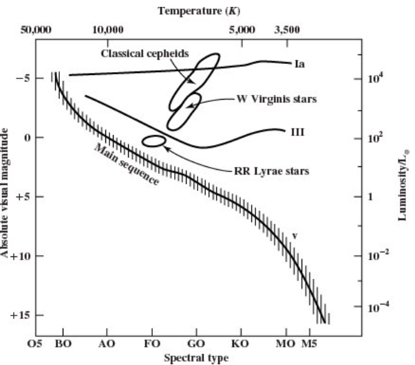
To study variable stars, astronomers create light curves, graphs of magnitude over time. Long-term monitoring is essential. Different variable star types are classified based on period and magnitude range, visible in different parts of the HR diagram.
Cepheid mechanism
Cepheid variables exhibit Doppler shifts in spectral lines that vary throughout their light cycle, indicating surface movement. These stars undergo radial oscillations involving inward and outward motions of outer layers. The luminosity changes are associated with alterations in surface temperature and radius. Cepheid variables typically form when a star reaches a specific stage in its evolution.
The oscillations in a normal star are radial, involving inward and outward motions of the outer layers. When perturbed by decreasing its radius R, the increased density and pressure cause the outer layers to expand, overshooting the equilibrium radius \(R_0\). As the star becomes larger than \(R_0\), pressure decreases, allowing material to fall back, repeating the process.
Ignoring opacity effects in a normal star, where opacity decreases with temperature, a perturbation with \(R < R_0\) causes increased pressure and temperature. The subsequent reduction in opacity allows excess pressure relief through heat flow, reducing the tendency to overshoot. Conversely, if perturbed with \(R > R_0\), decreased pressure and temperature, along with increased opacity, reduces the tendency to fall back too fast.
Opacity quenches oscillation in normal stars but, for specific conditions with opacity increasing as temperature rises (due to \(He^+\) ionization forming \(He^{++}\)), starting with \(R< R_0\) enhances the tendency to overshoot. Conversely, with \(R > R_0\), decreased pressure and temperature, coupled with reduced opacity, leads to material falling back quickly and overshooting. These conditions can sustain oscillations indefinitely, defining Cepheid variables.
Period–luminosity relation
Cepheids play a crucial role in distance measurement due to their period–luminosity relation. This relationship correlates the period and mean absolute magnitude of Cepheids, allowing astronomers to infer distances when observing their apparent magnitudes. The technique is particularly valuable for galaxies where Cepheids are bright enough to be observed.
Calibrating the period–luminosity relationship requires independent distance measurements for Cepheids, a challenge given their absence in proximity. Calibrations have been achieved through statistical studies.
An intriguing finding in the distribution of Cepheids is the presence of two peaks, indicating two types: classical Cepheids with shorter periods, and type II Cepheids or W Virginis stars with longer periods. Type II Cepheids are fainter than classical Cepheids, and their period–luminosity relation differs slightly.
Another type of variable star useful in distance determination is the RR Lyrae variable, cluster variables, exhibit short periods, and possess absolute magnitudes close to zero.
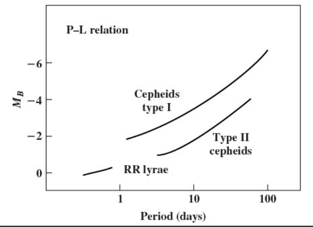
The existence of period–luminosity relations in pulsating stars is reasonable, given that for radial oscillations, the period is expected to be roughly proportional to (Gρ)(-1/2), where ρ is the average density of the star. This qualitative understanding is analogous to the period of a a pendulum, and the relation holds true in systems where gravity dominates.
Planetary nebulae
White dwarfs
The death of high mass stars
Higher-mass stars undergo significant mass loss, a crucial aspect of their evolutionary process. Mass shedding happens through winds or the expulsion of planetary nebulae, with substantial mass loss, possibly surpassing half of the initial mass, occurring as these stars advance toward the red supergiant phase. The trajectory of a star's evolution is influenced by its starting mass and the extent of mass loss experienced throughout its stellar journey.
Supernovae
Neutron stars
Pulsars
Stellar black holes
Special relativistic effects impose a limit on the mass sustained by neutron degeneracy pressure, much like in the case of electron degeneracy. The precise limit is uncertain, with neutron degeneracy alone supporting approximately \(2M_\odot\). Interactions among neutrons can raise this limit to around \(3M_\odot\), a commonly used figure, although some calculations propose it could be as high as \(8M_\odot\).
Regardless of the specific limit, if a neutron star exceeds it, stability cannot be maintained. In such cases, the star will inevitably collapse within its Schwarzschild radius, transforming into a black hole. Consequently, black holes seem to be a typical endpoint for stellar evolution, provided neutron stars are not formed with masses below about \(3M_\odot\). While isolated stellar black holes may be challenging to detect directly, their presence can be inferred through gravitational effects on other stars, particularly in binary systems.